Adventures in Recreational Mathematics VII: numbers not astronomical in size

Isky Mathews

Supplement №2, Volume II

Isky Mathews

]

This time we will examine some of mathematics’ largest numbers; I feel this is a conceptual area that many find interesting, and even amusing, to think about—some of the numbers I will mention here will be so large that to refer to them as astronomical would not just be inaccurate, since there is no object that could found in these quantities within the observable universe, but, frankly, insulting to their magnitude.

To demonstrate the previous point, we shall begin by considering the number of baryons in the observable universe. Baryons are particles made up of 3 quarks and interact with the strong nuclear force, e.g. protons or neutrons, and we can calculate how many there are using 4 numbers, 3 of which were obtained using data from the Planck Satellite:

• \(\rho_{crit}\), the critical density of the universe (\(=8.64\times10^{-33}kgm^{-3}\))

• \(\Omega_b\), the fraction of the universe’s energy in baryons (\(=0.0485\))

• \(L\), the radius of the observable universe, which is roughly spherical (\(=4.39\times10^{26}cm\))

• \(m_p\), the mass of one proton (\(=1.67\times10^{-27}kg\))

Now, since \(\rho_{crit}\) is essentially the energy density of the universe, \(\rho_{crit}\times\Omega_b\) is the mass stored in baryons per \(cm^3\) of the observable universe on average, making \(\rho_{crit}\times\Omega_b\times\frac{4}{3}\pi L^3\) roughly the combined mass of all baryons in the universe. Finally, since a neutron’s mass is essentially equivalent to that of a proton, we divide the above expression by \(m_p\) to get

\[\frac{\rho_{crit}\times\Omega_b\times\frac{4}{3}\pi L^3}{m_p} = 8.89\times10^{79}\]

which is really quite a big number, in comparison to the numbers of things you encounter for everyday life! However, it was small enough to be expressed, to a fair level of precision and concisely, using a notation we are so familiar with that I barely need to name it: that of the exponential. For many, if asked to write down quickly the biggest number they could think of at the time, exponentials or stacked exponentials¹ would be their first thought, since it’s so simple—for example, just \(10^{10^{2}}\) is bigger than the number of baryons in the universe. In fact, our first famous number can be expressed as \(10^{100}\), a googol, and the next as \(10^{10^{100}}\), a googolplex. We shall return to exponentials and the process of stacking them later, for it has great potential to make large numbers.

Primitive Recursive and Non-Primitive Recursive functions

For now, we take ourselves back to near the beginning of the 20th century, where individuals such as Gödel, Turing and Church were discussing the nature of functions. They realised that the process of calculating the outputs to most functions could be seen as an iterative process that, most importantly, had a predictable number of steps; for example, to calculate \(2+2\), one could see it as applying \(f(n) = n+1\) to the input \(2\) twice. Such functions were called primitive recursive, because they could be written down or represented recursively, i.e. where they were seen as a series of repeated applications of some function, but could also be written down in a single closed form—all polynomials, exponentials and many more that we are familiar with are primitive recursive. The computer scientist Robert Ackermann is most famous for describing an eponymous function, denoted \(A(m,n)\), that was still possible to evaluate but was not primitive recursive defined by these conditions:

\[A(m,n) = \begin{cases} \text{\(n+1\)} &\quad\text{if \(m=0\)}\\ \text{\(A(m-1,1\))} &\quad\text{if \(m>0\) and \(n=0\)}\\ \text{\(A(m-1, A(m, n-1))\)} &\quad\text{if \(m>0\) and \(n>0\)} \end{cases}\]
Let us call a closed-form representation of a function a form which uses a finite number of operations and without self reference. Then, an amazing fact is that the Ackermann function’s above self-referential or recursive definition cannot be written out into a closed form, unlike addition or multiplication—this is what it means for it to not be a primitve-recursive function and it grows extremely quickly—try evaluating it for different inputs! Clearly things like \(A(0, 3) = 4\) and \(A(1, 2) = 4\) are quite small, but then \(A(4,3)\) is an incredible 19729 digit number:

\[A(4,3) = 2^{2^{65536}}-3\]
In fact, it’s often difficult to find examples to demonstrate how large the numbers are that the Ackermann function outputs, because nearly all of them are so big that they either can’t be written down in any concise manner or, worse, they couldn’t be computed within the lifetime of the universe given all the computing available today. Furthermore, Ackermann and his peers were later able to show that functions of this kind² dominate all primitive recursive functions, i.e. for any primitive recursive function \(f(x)\) and a non-primitive-recursive function \(g(x)\), there is some input \(n\) so that for all \(m>n\), \(g(m) > f(m)\).

In order to understand and express just how quickly such functions grow, we have to use a lovely typographical system developed some years ago by the famous Donald Knuth³ known as up-arrow notation, which is based on the idea of the hyperoperation hierarchy. The first operator in the hierarchy is that of the successor, an unary operator (meaning that it takes 1 argument) which takes in \(n\) and outputs \(n+1\), often written \(n++\).⁴ Addition can be seen as repeated successorship in that \(a+b\) can be seen as denoting \(a++\), \(b\) times. Multiplication can then be seen as repeated addition in that \(a\times b\) represents \(a+a\), \(b\) times. This continues as we go higher up the hierarchy, with each \(n\)th operation \(a*_nb\) representing performing the \((n-1)\)th operation to \(a\) by itself, \(b\) times. Knuth created the hyperoperation-notation \(a\uparrow b\) which starts at exponentiation (as in \(a\uparrow b = a^b\)) and by writing more arrows, one goes up the hierarchy, so \(2 \uparrow \uparrow 4 = 2^{2^{2^{2}}}\)—the name we give for this operation above exponentiation is "tetration" and \(a \uparrow \uparrow \uparrow b\) is called "\(a\) pentated by \(b\)" etc. These operations make writing really large numbers simple and if we index the arrows, that is say that \(\uparrow^{n}\) denotes \(n\) arrows, then we can write down numbers that could never have any practical use—for example, the famous Graham’s number.

Graham’s Number

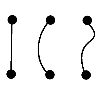
This number comes out of a question in a somewhat ill-defined area of mathematics known as Ramsey Theory, which purports to comprehend the conditions under which complex structures are forced to appear; Ronald Graham and Bruce Lee Rothschild, both legends in this field, came up with the question in 1970. The question requires understanding what a graph is in pure mathematics; Benedict Randall Shaw has written a helpful article explaining graph theory in a previous issue of The Librarian⁵, but a summary is that any set of points and lines drawn connecting them is a graph. More formally, a graph is a set of points along with a set of pairings defining connections between those points—thus neither the precise coordinate/relative position of points nor the shape of the lines connecting them matters, only the connections⁶.

Given \(n\) points, the graph obtained by adding all possible connections between them is called the complete graph on \(n\) vertices, denoted \(K_n\) (e.g. \(K_3\) is like a triangle and \(K_4\) is like a square with its diagonals drawn in). Now, Rothschild and Graham were considering complete graphs of \(n\)-dimensional cubes⁷, which have \(2^n\) vertices each, and properties of the colourings of their edges, i.e. the ways in which you can assign different colours to those edges. In particular, they asked what was the smallest value of \(n\) such that every 2-colour colouring, using, for example, red and blue, of the edges of the complete graph on an \(n\)-dimensional cube is forced to contain a subset \(S\) containing exactly 4 of its points such that all the edges between the points in \(S\) are the same colour and such that all points in \(S\) are coplanar⁸. They were able to prove that there is such an \(n\) and they knew from checking on paper that \(n>5\) and so they sought to also put an upper-bound on it (Graham’s number)⁹. It is constructed as follows:

• Let \(G_1 = 3 \uparrow^4 3\) (an amazingly large number, so big that the number of 3s in its power-tower representation couldn’t be written in base 10 even if each digit could be assigned to each planck-volume in the observable universe!)

• For each \(n\), let \(G_{n+1} = 3\uparrow^{G_n}3\)

• Then Graham’s number is \(G_{64}\).

It is clear from this that uparrow notation becomes inadequate for integers as large as Graham’s Number, since there is no way of expressing it concisely if we need to write out all the arrows. Thus, when you have gotten over \(G_{64}\), we must move on to a better framework that will allow us to see just how large it is "in the grand scheme of things".

The Fast-Growing Hierarchy or the Grandest of Schemes of Things

The fast-growing hierarchy is a series of functions, built recursively, that grow faster and faster as we go up. We start with the simple function \(f_0(x) := x+1\) and we say¹⁰ that \(f_1(x) := f_0^x(x)\), or in other words \(x+x\). Similarly, \(f_2(x) := f_1^x(x) = x\times x\) and in general for any integer \(n>0\), \(f_n(x) = f_{n-1}^x(x)\).

So far, there is no difference between this and hyperoperations but now, we can use ordinals to give us unbounded growth-rates…There was a previous article¹¹ introducing readers to the wonderful universe of ordinals but, to simplify their technical definition, they are a clever set-theoretic version of numbers, discovered by Georg Cantor, which essentially allows us to have a natural extension of the integers to varying sizes of infinity. The number \(\omega\) is the ordinal "larger" than all the integers but then we still have a well-defined concept of \(\omega+1\) or \(+2\) or \(+n\) and much, much more. We call \(\omega\) the first limit ordinal, meaning that it has no specific predecessor, but rather can be reached as a limit of a strictly increasing sequence, and we call \(2, 3, 4,n, \ldots\) and \(\omega+1, \omega+2,\omega+n\) etc. successor ordinals because they do have a well-defined predecessor (i.e. they are the successor of some known ordinal). Thus we have the definition that if \(\alpha\) is a successor ordinal, then \(f_\alpha(x) = f_{\alpha-1}^x(x)\), and if \(\alpha\) is a limit ordinal and \(S_\alpha\) is a strictly-increasing sequence of ordinals whose limit is \(\alpha\) (as in, \(\alpha\) is the smallest upper-bound for all the terms in \(S_\alpha\)), with \(S_{\alpha} [n]\) denoting the \(n\)th term of \(S_\alpha\) for some ordinal \(n\), then \(f_\alpha(x) = f_{S_{\alpha}}[x](x)\).

To give an example¹², \(f_\omega(x) = f_x(x)\), since the sequence of integers 1,2,3,…,\(x\),…has the limit \(\omega\) but since \(\omega+1\) is a successor ordinal, \(f_{\omega+1}=f_\omega^x(x)\). We can observe from these definitions immediately that \(f_\omega(x)\) can’t be primitive-recursive, since it grows faster than any \(f_n\) for integer \(n\), and thus that it is, in a sense, beyond uparrows, since it can’t be represented in the form \(m \uparrow^k x\), where \(m,k\) are fixed integers. In fact, it is possible to show that \(f_\omega(x)\) grows at almost exactly the same rate as the Ackermann function that we’ve seen previously and that \(f_{\omega+1}(64) > G_{64}\).¹³ Now, you can choose your favourite transfinite ordinal and create a function that grows faster than you can imagine, for example \(f_{\omega\times2}, f_{\omega^2}, f_{\omega^\omega}\) or, if \(\epsilon_0 = \omega^{\omega^{\omega^{\omega^{\ldots}}}}\), then you can even have \(f_{\epsilon_0}\) and larger!