Adventures in Recreational Mathematics VIII—in full: Numbers that are not astronomical

Isky Mathews

Supplement №3, Volume II

This time we will examine some of mathematics’ largest numbers; I feel this is a conceptual area that many find interesting, and even amusing, to think about—some of the numbers I will mention here will be so large that to refer to them as astronomical would not just be inaccurate, since there is no object that could found in these quantities within the observable universe, but, frankly, insulting to their magnitude.

To demonstrate the previous point, we shall begin by considering the number of baryons in the observable universe. Baryons are particles made up of 3 quarks and interact with the strong nuclear force, e.g. protons or neutrons, and we can calculate how many there are using 4 numbers, 3 of which were obtained using data from the Planck Satellite:

• \(\rho_{crit}\), the critical density of the universe (\(=8.64\times10^{-33}kgm^{-3}\))

• \(\Omega_b\), the fraction of the universe’s energy in baryons (\(=0.0485\))

• \(L\), the radius of the observable universe, which is roughly spherical (\(=4.39\times10^{26}cm\))

• \(m_p\), the mass of one proton (\(=1.67\times10^{-27}kg\))

Now, as \(\rho_{crit}\) is essentially the energy density of the universe, \(\rho_{crit}\times\Omega_b\) is the mass stored in baryons per \(cm^3\) of the observable universe on average, making \(\rho_{crit}\times\Omega_b\times\frac{4}{3}\pi L^3\) roughly the combined mass of all baryons in the universe. Finally, because a neutron’s mass is essentially equivalent to that of a proton, we divide the above expression by \(m_p\) to get

\[\frac{\rho_{crit}\times\Omega_b\times\frac{4}{3}\pi L^3}{m_p} = 8.89\times10^{79}\]

which is really quite a big number, in comparison to the numbers of things you encounter in everyday life. However, it was small enough to be expressed, to a fair level of precision and concisely, using a notation with which we are so familiar that I barely need to name it: that of the exponential. For many, if asked to write down quickly the biggest number they could think of at the time, exponentials or stacked exponentials of the form

\[a^{b^{c^{d^{\ldots}}}}\]

would be their first thought, due to its simplicity—for example, just \(10^{10^{2}}\) is more than the number of baryons in the universe. In fact, our first famous number can be expressed as \(10^{100}\), a googol, and the next as \(10^{10^{100}}\), a googolplex. We shall return to exponentials and the process of stacking them later, for it has great potential to make large numbers.

Primitive Recursive and Non-Primitive Recursive functions

For now, we take ourselves back to near the beginning of the 20th century, when individuals such as Gödel, Turing and Church were discussing the nature of functions. They realised that the process of calculating the outputs to most functions could be seen as an iterative process that, most importantly, had a predictable number of steps; for example, to calculate \(2+2\), one could see it as applying \(f(n) = n+1\) to the input \(2\) twice. Such functions were called primitive recursive, because they could be written down or represented recursively, i.e. where they were seen as a series of repeated applications of some function, but could also be written down in a single closed form—all polynomials, exponentials and many more that we are familiar with are primitive recursive. The computer scientist Robert Ackermann is most famous for describing an eponymous function, denoted \(A(m,n)\), that was still possible to evaluate but was not primitive recursive, defined by these conditions:

\[A(m,n) = \begin{cases} \text{\(n+1\)} &\quad\text{if \(m=0\)}\\ \text{\(A(m-1,1\))} &\quad\text{if \(m>0\) and \(n=0\)}\\ \text{\(A(m-1, A(m, n-1))\)} &\quad\text{if \(m>0\) and \(n>0\)} \end{cases}\]
Let us call a closed-form representation of a function a form which uses a finite number of operations and without self reference. Then, an amazing fact is that the Ackermann function’s above self-referential or recursive definition cannot be written out into a closed form, unlike addition or multiplication—this means it is not a primitive-recursive function and it grows extremely quickly—try evaluating it for different inputs! Clearly things like \(A(0, 3) = 4\) and \(A(1, 2) = 4\) are quite small, but then \(A(4,3)\) is an incredible 19729 digit number:

\[A(4,3) = 2^{2^{65536}}-3\]
In fact, it’s often difficult to find examples to demonstrate how large the numbers that the Ackermann function outputs are, because nearly all of them are so big that they either can’t be written down in any concise manner or, worse, they couldn’t be computed within the lifetime of the universe given all the computing available today. Furthermore, Ackermann and his peers were later able to show that functions of this kind¹ dominate all primitive recursive functions, i.e. for any primitive recursive function \(f(x)\) and a non-primitive-recursive function \(g(x)\), there is some input \(n\) so that for all \(m>n\), \(g(m) > f(m)\).

In order to understand and express just how quickly such functions grow, we have to use a lovely notation developed some years ago by the famous Donald Knuth² known as up-arrow notation, which is based on the idea of the hyperoperation hierarchy. The first operator in the hierarchy is the successor, an unary operator (meaning that it takes 1 argument) which takes in \(n\) and outputs \(n+1\), often written \(n++\).³ Addition can be seen as repeated successorship in that \(a+b\) can be seen as denoting \(\ldots{}((a++)++)++\ldots{}\), where the successor operation is applied \(b\) times. Similarly, multiplication is repeated addition, as \(a\cdot b\) is equal to \(a+a\ldots+a\) where \(a\) appears \(b\) times. We can make a hierarchy of such functions, with \(a*_1 b=a\cdot b\) by definition, and thereafter, \(a*_n b\) defined as \(a*_{n-1}(a*)\) with \(b\) instances of \(a\) in that definition. Knuth created the hyperoperation-notation \(a\uparrow b\) which starts at exponentiation (as in \(a\uparrow b = a^b\)) and by writing more arrows, one goes up the hierarchy, so \(2 \uparrow \uparrow 4 = 2^{2^{2^{2}}}\)—the name we give for this operation above exponentiation is "tetration" and \(a \uparrow \uparrow \uparrow b\) is called "\(a\) pentated by \(b\)" etc. These operations make writing really large numbers simple and if we index the arrows, that is say that \(\uparrow^{n}\) denotes \(n\) arrows, then we can write down numbers that could never have any practical use—for example, the famous Graham’s number.

Graham’s Number

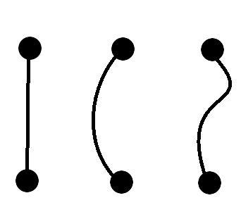
This number comes out of a question in a somewhat ill-defined area of mathematics known as Ramsey Theory, which purports to comprehend the conditions under which complex structures are forced to appear; Ronald Graham and Bruce Lee Rothschild, both legends in this field, came up with the question in 1970. The question requires understanding what a graph is in pure mathematics; Benedict Randall Shaw has written a helpful article explaining graph theory in a previous issue of The Librarian⁴, but a summary is that any set of points and lines drawn connecting them is a graph. More formally, a graph is a set of points along with a set of pairings defining connections between those points—thus neither the precise coordinate/relative position of points nor the shape of the lines connecting them matters, only the connections⁵.

Given \(n\) points, the graph obtained by adding all possible connections between them is called the complete graph on \(n\) vertices, denoted \(K_n\) (e.g. \(K_3\) is like a triangle and \(K_4\) is like a square with its diagonals drawn in). Now, Rothschild and Graham were considering complete graphs on \(n\)-dimensional cubes⁶, which have \(2^n\) vertices each, and properties of the colourings of their edges, i.e. the ways in which you can assign different colours to those edges. In particular, they asked what was the smallest value of \(n\) such that every 2-colour colouring, using, for example, red and blue, of the edges of the complete graph on an \(n\)-dimensional cube is forced to contain a subset \(S\) containing exactly 4 of its points such that all the edges between the points in \(S\) are the same colour and such that all points in \(S\) are coplanar⁷. They were able to prove that there is such an \(n\), and they knew from checking on paper that \(n>5\), and so they sought to also put an upper-bound on it (Graham’s number)⁸. It is constructed as follows:

• Let \(G_1 = 3 \uparrow^4 3\) (an amazingly large number, so big that the number of 3s in its power-tower representation couldn’t be written in base 10 even if each digit could be assigned to each planck-volume in the observable universe!)

• For each \(n\), let \(G_{n+1} = 3\uparrow^{G_n}3\)

• Then Graham’s number is \(G_{64}\).

It is clear from this that uparrow notation becomes inadequate for integers as large as Graham’s Number, since there is no way of expressing it concisely if we need to write out all the arrows. Thus, when you have gotten over \(G_{64}\), we must move on to a better framework that will allow us to see just how large it is "in the grand scheme of things".

The Fast-Growing Hierarchy or the Grandest of Schemes of Things

The fast-growing hierarchy is a series of functions, built recursively, that grow faster and faster as we go up. We start with the simple function \(f_0(x) := x+1\) and we say⁹ that \(f_1(x) := f_0^x(x)\), or in other words \(x+x\). Similarly, \(f_2(x) := f_1^x(x) = x\times x\) and in general for any integer \(n>0\), \(f_n(x) = f_{n-1}^x(x)\).

So far, there is no difference between this and hyperoperations but now, we can use ordinals to give us unbounded growth-rates…There was a previous article¹⁰ introducing readers to the wonderful universe of ordinals but, to simplify their technical definition, they are a clever set-theoretic version of numbers, discovered by Georg Cantor, which essentially allows us to have a natural extension of the integers to varying sizes of infinity. The number \(\omega\) is the ordinal "larger" than all the integers but then we still have a well-defined concept of \(\omega+1\) or \(+2\) or \(+n\) and much, much more. We call \(\omega\) the first limit ordinal, meaning that it has no specific predecessor, but rather can be reached as a limit of a strictly increasing sequence, and we call \(2, 3, 4,n, \ldots\) and \(\omega+1, \omega+2,\omega+n\) etc. successor ordinals because they do have a well-defined predecessor (i.e. they are the successor of some known ordinal). Thus we have the definition that if \(\alpha\) is a successor ordinal, then \(f_\alpha(x) = f_{\alpha-1}^x(x)\), and if \(\alpha\) is a limit ordinal and \(S_\alpha\) is a strictly-increasing sequence of ordinals whose limit is \(\alpha\) (as in, \(\alpha\) is the smallest upper-bound for all the terms in \(S_\alpha\)), with \(S_{\alpha} [n]\) denoting the \(n\)th term of \(S_\alpha\) for some ordinal \(n\), then \(f_\alpha(x) = f_{S_{\alpha[x]}}(x)\).

To give an example¹¹, \(f_\omega(x) = f_x(x)\), since the sequence of integers 1,2,3,…,\(x\),…has the limit \(\omega\) but since \(\omega+1\) is a successor ordinal, \(f_{\omega+1}=f_\omega^x(x)\). We can observe from these definitions immediately that \(f_\omega(x)\) can’t be primitive-recursive, since it grows faster than any \(f_n\) for integer \(n\), and thus that it is, in a sense, beyond uparrows, since it can’t be represented in the form \(m \uparrow^k x\), where \(m,k\) are fixed integers. In fact, it is possible to show that \(f_\omega(x)\) grows at almost exactly the same rate as the Ackermann function that we’ve seen previously and that \(f_{\omega+1}(64) > G_{64}\).¹² Now, you can choose your favourite transfinite ordinal and create a function that grows faster than you can imagine, for example \(f_{\omega\times2}, f_{\omega^2}, f_{\omega^\omega}\) or, if \(\epsilon_0 = \omega^{\omega^{\omega^{\omega^{\ldots}}}}\), then you can even have \(f_{\epsilon_0}\) and larger!

Kruskal’s Tree Theorem and \(TREE(3)\)

Kruskal’s Tree Theorem, conjectured by Andrew Vazsonyi and proved in 1960 by Joseph Kruskal (an influential combinatoricist), is a statement, once again, relating to graphs and to explain it, we need some more vocabulary concerning them.

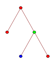
We say that, given a graph \(G\) and a point \(p\) in \(G\), if there is a way of starting at \(p\) and traversing a finite number of edges (that is greater than 2) to move through a sequence of distinct vertices of \(G\) which eventually ends up at \(p\) again, then we call such a path a cycle and we call a graph acyclic if it doesn’t doesn’t contain any cycles. Connected graphs are what they sound like—they are graphs with the property that for any two of its vertices, there is always a path between them. Further, we say that a connected, acyclic graph \(G\) that is also rooted, i.e. there is one vertex we call the root and every other vertex is considered (and often drawn) "below" that root, is called a tree. This makes sense intuitively and Fig. 1 gives an example of a tree to demonstrate. Similarly, peiople call the vertices at the ends of branches of trees leaves and, if one vertex \(v_1\) is closer to the root than \(v_2\) and their paths to the root overlap, then we call \(v_1\) a parent of \(v_2\).

A \(k\)-labeled tree is one where each of the tree’s vertices are assigned one of \(k\) "labels", which for our purposes we may consider as colours. The most complicated definition that Kruskal’s Theorem requires us to consider is the idea of a \(k\)-labeled tree \(T_1\) being homeomorphically embeddable (h.e. from now on) into another \(k\)-labeled tree \(T_2\). Given \(T_1\) and \(T_2\), we say that \(T_1\) can be h.e. into \(T_2\) if there is a function \(p(x)\) that takes as inputs vertices of \(T_1\) and outputs vertices of \(T_2\) with the properties that

• for every vertex \(v\) from \(T_1\), \(v\) and \(p(v)\) have the same colour;

• for every pair of vertices \(v_1, v_2\) from \(T_1\) and if \(x ANC y\) denotes the closest common parent of two vertices \(x\) and \(y\), then \(p(v_1 ANC v_2)\) has the same colour as \(p(v_1) ANC p(V_2)\).

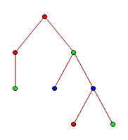
To illustrate this somewhat abstract definition, you can look at Fig. 3 which gives an example of two \(k\)-labeled trees with the first being h.e. into the other. Finally, Kruskal’s Tree Theorem states that for any \(k\) and for any infinite sequence of \(k\)-labelled trees \(T_1, T_2, T_3, ...\), where each \(T_n\) can have at most \(n\) vertices, it is true that for some \(i\) and some \(j>i\), the tree \(T_i\) is h.e. into \(T_j\). While the theorem itself doesn’t allow us to describe large numbers, the mathematician Harvey Friedman made the observation that the theorem allows us to define the function \(TREE(n)\), which returns the length of the longest finite sequence of \(n\)-labeled trees such that no \(T_i\) is h.e. into a \(T_j\) for integers \(i\) and \(j>i\) and it turns out that \(k\)-labellings of trees are amazingly combinatorially rich:

• \(TREE(1) = 1\), since \(T_1\) can have at most 1 vertex and at most use 1 colour, so it is simply a single coloured point and that is clearly h.e. into any successive trees of the same colour.

• \(TREE(2) = 3\), where the sequence begins with a single vertex of Colour 1, then we have a two-vertex tree of Colour 2 and then we have a single vertex of Colour 2—can you see why this is the longest such sequence?

• \(TREE(3)\) then is so vastly, incredibly large that I struggle to find description for it.

The first thing we can say is that an extremely lower bound that can be proven for it is \(f_\omega^{f_\omega(187196)}(2)\), which is clearly immensely bigger than \(f_{\omega+1}(64)>G_64\)! I shall now attempt to explain how far up one needs to go in the fast-growing hierarchy to reach a function that can rival \(TREE(n)\).

In the 20th century, the mathematician Veblen, along with others, was attempting to create a schema for notating and comparing really large infinite ordinals; he first proved that if one has a function \(h(x)\) that takes as inputs and outputs ordinals, that is strictly increasing, and whose value for a limit ordinal \(\lambda\) is equivalent to the limit of the sequence \(h(a_0), h(a_1), h(a_2), ...\) where the limit of \(a_0, a_1, a_2, ...\) is \(\lambda\),¹³ then \(h(x)\) has fixed points for some ordinals. This remarkable property of the ordinals is part of what makes them so interesting to study for set-theorists—they seem to be "averse" to notation systems for them. Regardless, Veblen created his Veblen hierarchy, a series of functions \(\phi_0(x), \phi_1(x), \phi_2(x), ...\) where \(\phi_0(x) = \omega^x\) and each \(\phi_{n+1}(x)\) is equal to the \(x\)th fixed point of \(\phi_n(x)\)—take \(\phi_1(1)\), for example, which is the first fixed point of \(\omega^{x}\), i.e. \(\epsilon_0\) as discussed previously. Now, the Feferman-Schütte ordinal \(\Gamma_0\) is the smallest ordinal \(\alpha\) that satisfies the impressive \(\phi_\alpha(0) = \alpha\) or, to paraphrase Solomon Feferman himself, \(\Gamma_0\) is the smallest ordinal that cannot be reached by starting with 0 and repeatedly using addition and the Veblen hierarchy of functions¹⁴ (in fact, it is very difficult to create notation systems that can describe ordinals above \(\Gamma_0\) as well as all those below it).

What we can now explain is that despite the magnitude of \(\Gamma_0\), it is possible to show that the growth rate of \(TREE(n)\) is much greater than that of \(f_{\Gamma_0}(x)\). But, ultimately, \(TREE(n)\) is piffle in comparison to what comes next—after all, it grows slow enough for it to still be computable...

Computability and busy beaver numbers

You recall the distinction between recursive and primitive-recursive functions made by those great minds near the beginning of the 20th century? That result is but one in a bigger theory of computation called, aptly, computability theory. Computability theorists study fundamentally what it means to compute something by examining models of computation.

Mathematicians in this era were attempting to go back to the foundations of mathematics and to formalise them, that is to make them completely logically rigorous and unambiguous—this was because it had been discovered that without such careful thought and by relying on implicit or vague definitions, one can run into paradoxes or questions that don’t have an answer, simply because they don’t mean anything. One of the interesting notions that Church and Turing picked up on this journey was that most people appeared to assume that all functions and questions in mathematics were answerable and simply required "proper definitions" and a great amount of thought—their great insight was that the process of logically working things out or deducing true statements had mathematical properties in and of itself and thus realised that it was possible to create problems that were well defined (as in, they had a unique answer) but were beyond the capability of any proof-system or computational device to solve; such problems are known as uncomputable problems.

Computability theory is such an amazing area of mathematics that it deserves its own article¹⁵ but we shall simplify here to explain just the concepts required for describing large numbers. Alan Turing came up with the concept of Turing machine (tms from now on), which are theoretical automata that have a tape that stretches out infinitely in one direction and is divided up into discrete tape-segments, along with a tape-head that is capable of reading and writing symbols on the tape.

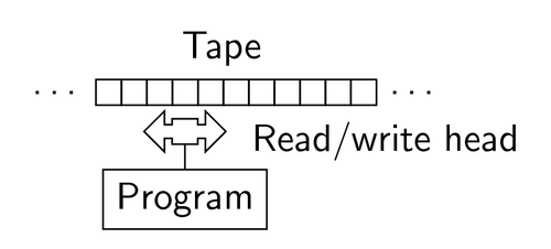
It also has a number of states that it can be in and a rulebook that determines, given that the tm is in the \(n\)th state and that the symbol being read by the tape-head is \(X\), what symbol \(Y\) the tm should overwrite \(X\) with and whether to then move one tape-segment right or left. It should finally be noted that a tm has two special states denoted \(YES\) or \(NO\) which, when reached during some stage of a tm-computation, cause the tm to halt, i.e. cease all movement. Turing and Church believed that a Turing machine should be able to perform any algorithm that is well-defined because:

• They (and other mathematicians such as Gödel) had previously created other systems which were supposed to represent computation, such as the \(\lambda\)-calculus and the set of general recursive functions, and it turned out that the set of problems they could solve were all equivalent.

• They were able to show ways of creating Turing machines that could evaluate many well known algorithms, such as one that could perform primality-checks or could multiply two numbers together.

• They lived to see John von Neumann, a startingly brilliant mind, design modern-day computer architectures using their ideas and create the first computers.

In fact, in the 1960s and 70s, many individuals tried to create other deterministic systems that they believed might be able to compute more than Turing machines but all were eventually proved to be able to solve the same set of problems—thus, they proposed the Church-Turing thesis: that every sequence of logical steps that were performable by a human would also be performable, theoretically, by a Turing machine, and vice versa; subsequently, any system that was capable of solving the same set of problems as tms came to be known as Turing-complete.

However, as I mentioned previously, those problems Turing-complete systems can solve do not encompass all problems, they only contain computable problems. But what, then, would an uncomputable problem look like? Well, Turing made the observation that certain Turing machines are setup such that, after some finite number of steps, they halt in the state \(YES\) or \(NO\) and others never halt and simply continue moving along their tape indefinitely. In 1936, he published a paper describing the Halting problem’s uncomputability: it is impossible to create a general, finite-time algorithm to decide accurately whether a given tm halts—he showed this through a clever proof-by-contradiction. To illustrate it, we first remember that, by Turing-completeness, any computability theorem that applies to Turing machines applies to many of the modern-day computer programming languages¹⁶, so we shall precede by writing our proof in the language of Python. Let us assume, hoping to reach a contradiction, that there was a program defining a function called Halts(\(x\))—this takes in the name of a programmed-function for which you wish to check whether it halts or not and outputs after a finite amount of time either True or False as per the answer. Then consider the function:

For those less familiar with Python, contradiction(x) is designed to halt after a finite amount of time if and only if Halts(\(x\)) says that it will run forever and contradiction(x) will loop forever if and only if Halts(\(x\)) says that it will halt after a finite amount of time. This function is clearly contradictory and so our initial assumption, that there could exist such a function Halts(\(x\)), is false. Thus, the Halting problem is uncomputable!

An interesting observation, then, made by a researcher at Bell Labs was that, for a given \(n\), it must be true that there is some number \(k\) representing the largest number of steps that a halting \(n\)-state Turing machine (i.e. a tm which does eventually terminate its computation) will take before stopping—the researcher called these tms Busy Beavers and the corresponding \(k\) for each \(n\) the \(n\)th Busy Beaver number (\(BB(n)\)), because they take a long time to stop and the way that they move up and down their tape during their computation reminded him of a beaver making a dam. So, by definition, there is no \(n\)-state Turing machine that takes longer than \(BB(n)\) steps to halt.

However, he pointed out that there cannot exist a general algorithm to compute \(BB(n)\) for each input \(n\) because if there was one, then we would have the following finite-time algorithm to solve the Halting problem:

• If the tm for which we are trying to determine whether it halts or not has \(n\) states, compute \(BB(n)\).

• Then, start running the tm and wait \(BB(n)\) steps. If the tm halts by this time, then we know that it halts. If the tm does not halt by this time, then we know, by the definition of \(BB(n)\), that it does not halt.

but such an algorithm cannot exist by the uncomputability of the Halting problem and so \(BB(n)\) is an uncomputable function. Further, there cannot be any computable function \(g(n)\) which acts as an upper-bound to \(BB(n)\) for each \(n\), because if that was true then similarly we could wait \(g(n)\) steps to determine whether an \(n\)-state tm halts (any tm which takes longer than \(g(n)\) steps to halt must have already taken more than \(BB(n)\) steps, and so cannot halt), giving us again an impossible finite-time algorithm to solve the Halting problem. So, \(BB(n)\) isn’t just uncomputable—no computable functions can act as an upper-bound to it. So all the functions we have seen previously—\(A(m,n), f_\omega(n), f_{\epsilon_0}(n), f_{\Gamma_0}(n), TREE(n)\)—they all must inherently grow slower than \(BB(n)\) simply by the fact that they are computable.

Mathematicians have worked out that \(BB(0) = 0, BB(1) = 1, BB(2) = 4, BB(3) = 6\) and that \(BB(13)\) simply by trying and examining all \(n\)-state Turing machines for \(n<5\) but only lower bounds are known beyond this—for example, we know that

\[BB(7) > 10^{10^{10^{10^{18705353}}}}\]
and that

\[(BB(5) > 3^{3^{3^{3^{3^{...}}}}}\]
where the number of threes is 7625597484987.

But now we can go further even than this to functions and numbers so fantastic that I will at the end write down a number that, to my current knowledge, is greater than anything ever written in any mathematics publication, formal or informal as it is something of my own design. Because computability theory is all about imagining theoretical scenarios related to computation that could never happen—for example, we could never build an actual tm, since it requires an infinitely long tape—one thing we can consider is an oracle, a purely theoretical construct that would allow us to compute certain uncomputable functions. For example, we could have the oracle \(BB_0(n)\), which outputs the \(n\)th Busy Beaver number, although such a thing could never normally exist in our universe even if it was infinite but remember, this is pure mathematics—oracles can exist because we say so and they have interesting theoretical properties. For example, if you take the set \(S_0\) of tms equipped each with \(BB_0(n)\), the analogous version of the halting problem for \(S_0\) is still uncomputable by those tms in \(S_0\) and so \(S_0\) has its own associated Busy Beaver function, \(BB_1(n)\), that grows faster than any function computable by \(S_0\) tms (and thus grows far faster than \(BB_0(n)\)). Similarly, we could then introduce an oracle for \(BB_1(n)\) and create a new set of Turing machines \(S_1\) equipped with both the \(BB_1(n), BB_0(n)\) oracles and, once again, \(S_1\) would have its own version of the Halting Problem and thus a well-defined, but uncomputable function \(BB_2(n)\) that grows even faster than \(BB_1(n)\).

By iteratively creating more and more sets \(S_0, S_1, S_2, ...\), we get faster and faster growing functions assigned to them \(B_0(n),B_1(n),B_2(n),...\) and so, as with the fast-growing hierarchy, we can allow for ordinal subscripts where if \(\lambda\) is a limit ordinal, then \(B_\lambda(n)\) is the Busy Beaver function for Turing machines with oracles for all ordinals below it. Thus, we can have \(B_\omega(n)\) and \(B_{\epsilon_0}(n)\) etc. Now, we call an ordinal \(\alpha\) computable if there is a Turing machine which can tell for any two distinct ordinals \(\beta, \gamma\) smaller than \(\alpha\) whether \(\beta > \gamma\) or \(\gamma > \beta\) (for example, \(\omega\) is a computable ordinal, since any good computer can tell, given two nonequal integers, which one is bigger than the other). So, I define the Ultra-function \(U(n)\) to be \(B_{\delta(n)}(n)\), where \(\delta(n)\) is the largest ordinal computable for \(n\)-state Turing machines - so \(U(n)\) grows faster than any individual \(B_\alpha(n)\)!

Thus, as a final answer to Who can name the bigger number?, I advise you to simply write down \(K_{\Omega} = U(TREE(TREE(TREE(3))))\), which is quite concise but which I can verify, thanks to some results on much smaller numbers, is so big that if your opponent attempts to describe another number \(N\), whether the statement \(N>K\) is true is in fact independent of \(ZFC\)-set-theory (i.e. cannot be proved or disproved using most modern-day mathematical techniques, regardless of whether it seems obvious).

If you enjoyed this article and would interested in reading more, here are some titles of subjects and numbers that you can look up for further reading:

• Rayo’s Number (before I wrote \(K_{\Omega}\)’s definition above, it was the biggest number ever written down in human history)

• Chaitin’s constant, the Halting Problem and other uncomputable problems.

• Ordinals and Cardinals in Set Theory.

• Ramsey Theory and Ramsey Numbers.

• Go to the Googology Wiki, a fun website dedicated to listing and describing some of the largest numbers mathematicians know of!

And now for the challenges. For those who haven’t read ARM before, each article ends with 2 challenges and if you get a solution to either one, please email either Isky Mathews (isky.mathews@westminster.org.uk) or Benedict Randall Shaw (benedict.randallshaw@westminster.org.uk):

Challenge 1: Determine whether \(10^6\uparrow\uparrow10^6 > 3\uparrow\uparrow\uparrow 3\) or \(3\uparrow\uparrow\uparrow 3 >10^6\uparrow\uparrow10^6\).

Challenge 2: Can you think of a way of describing bigger numbers than using the "uncomputability hierarchy" above along with some form of (minimally-heuristic) argument as to why you believe they are bigger? (This would be exceedingly impressive, not just to us but to the entire mathematics community.)